Chapter 3 Session 3
In this session we will learn:
- lists, another data structure
- Classes
- the DGEList object from the package limma
3.1 Lists
Recall that we have previously learnt about the data structures: vectors, matrices and dataframes. Another important data structure is the list. Like a vector, it is 1 dimensional i.e. one row of data. Unlike vectors, you can put several data types in a list. Here, our list includes data of the integer, a character and a double types:
list(1, "a", 1.5)## [[1]]
## [1] 1
##
## [[2]]
## [1] "a"
##
## [[3]]
## [1] 1.5Not only can you put different data types into a list, you can also put a WHOLE data structure into one element of a list. In the list below, the first element is a vector that contains 3 numbers, the second element is a character and the third element is a dataframe that has two columns.
list(c(1,2,3),
     c("words", "letters"),
     data.frame(column1 = c(1,2,3), column2 = c("a","b","c"))
     )
## [[1]]
## [1] 1 2 3
##
## [[2]]
## [1] "words" "letters"
##
## [[3]]
## column1 column2
## 1 1 a
## 2 2 b
## 3 3 cThe output can often help you understand how the list is structured. The double brackets (e.g. [[1]]) signifies an element of the list and which index it is at. Here there are three elements in our list so the numbers in the double square brackets go from 1 to 3. Underneath the [[1]] and [[2]], there is a [1] - this indicates that the first and second elements both contain a vector. Underneath [[3]] you see the standard output for a dataframe, which we have seen before.
You even include a list within a list (within a list, within a list….I call this ‘list - ception’). This is where it starts to get confusing.
list(1, list(1,"a"))## [[1]]
## [1] 1
##
## [[2]]
## [[2]][[1]]
## [1] 1
##
## [[2]][[2]]
## [1] "a"- The first element, indicated by
[[1]], is a vector, indicated by the[1]underneath. - The second element, indicated by the first
[[2]]contains a list:[[2]][[1]]- tells you that the second element is a list, of which the first element of the inner list is the number 1.[[2]][[2]]- tells you that the second element is a list, of which the second element of the inner list is “a”.
Many bioconductor packages, including limma, use lists so it is an important data structure to understand.
Challenge 3.1
Below is the output from a list.
How many element of the list are there?
Look carefully at each element and answer the following questions about EVERY element of the list:
- How many elements does the element of the list contain?
- If there are several elements within this element, what does each element contain?
## [[1]]
## [[1]][[1]]
## [1] 1 2
##
## [[1]][[2]]
## [1] "b"
##
##
## [[2]]
## [1] "a" "b"
##
## [[3]]
## [[3]][[1]]
## [[3]][[1]][[1]]
## [1] "a"
##
## [[3]][[1]][[2]]
## [1] 1
##
##
## [[3]][[2]]
## [1] "b"
##
##
## [[4]]
## [1] "end"
We can access elements of a list using square brackets. You may have noticed that there are often double square brackets [[ ]]. There is a subtle but important difference between single square brackets and double square brackets when subsetting lists.
Let’s make a list:
my_list <- list(
  c("a","b"),
  c(1,2,3),
  c(4,5,6)
  )
Take a look at the output of obtaining the first element with single square brackets and double square brackets:
my_list[1]## [[1]]
## [1] "a" "b"my_list[[1]]## [1] "a" "b"The difference is minor; with my_list[1] there is an extra [[1]] at the top, with my_list[[1]] there is no [[1]] at the top.
The str() function gives us some more information:
str(my_list[1])## List of 1
## $ : chr [1:2] "a" "b"str(my_list[[1]])## chr [1:2] "a" "b"This tells us that when you use single brackets, the output is a list containing one element, which is a vector. When you use double brackets, the output is just a vector, NOT contained within a list.
Let’s use an analogy to gain a better understanding of this concept. Below is a picture of a cargo train, which contains a box in each segment. This represents a list containing 3 elements, with each element being the box.

Figure 3.1: Cargo train representation of a list.
Using a single bracket returns you the train segment with the box inside.
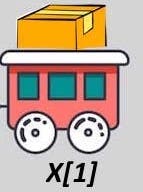
Figure 3.2: Single brackets with our cargo train list.
Using double brackets returns you just the box inside.
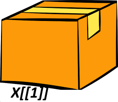
Figure 3.3: Double brackets with our cargo train list.
Back to our list:
my_list## [[1]]
## [1] "a" "b"
##
## [[2]]
## [1] 1 2 3
##
## [[3]]
## [1] 4 5 6To obtain the first element of the vector contained within the first element of the list (the "a") you can use:
my_list[[1]][1]## [1] "a"The [[1]] gives you just the vector contained within the first element of the list:
my_list[[1]]## [1] "a" "b"The second square bracket [1] then gives you the first element of the vector:
my_list[[1]][1]## [1] "a"Challenge 3.2
First create a new list:
my_list2 <- list(
  c("a","b"),
  c(1,2,3),
  data.frame(Name = c("Sally", "Andy"), Age = c(40,32))
  )
my_list2
## [[1]]
## [1] "a" "b"
##
## [[2]]
## [1] 1 2 3
##
## [[3]]
##    Name Age
## 1 Sally  40
## 2 Andy 32Subset this list to obtain a data structure that gives the following outputs:
## [1] "a" "b"## [1] "b"## [[1]]
## [1] 1 2 3## [1] 40## Name Age
## 1 Sally 40## [[1]]
## Name Age
## 1 Sally 40
## 2 Andy 323.1.1 Named list
You can also have names for each element of your list:
named_list <- list(
  name = c("Andy", "Sally"),
  age = c(32,40)
)
named_list
## $name
## [1] "Andy" "Sally"
##
## $age
## [1] 32 40If your list is named, you can use $ to access each element of your list:
named_list$name## [1] "Andy" "Sally"Note that the output is just the vector, NOT a vector within a list. Thus named_list[[1]] does the same thing as named_list$name.
Recall that we access columns in dataframes with the $ symbol as well. This means that if you have a dataframe within a list, you can obtain a column within the dataframe that is within the list using two $’s:
Let’s start with a list that contains a dataframe as its first element
named_list2 <- list(
 details = data.frame(name = c("Andy", "Sally"),
                      age = c(32,40))
)
named_list2
## $details
## name age
## 1 Andy 32
## 2 Sally 40We can get the age column using:
named_list2$details$age## [1] 32 40Extra:The reason you can also access columns in a dataframe with $ is because ‘under the hood’ a dataframe is actually a list. It is a list with the constraint that each element is a vector of the same length. Each element in the list is thus a column in the ‘dataframe’.
Challenge 3.3
Take a look at the named list below:
named_list3 <- list(
  cats = data.frame(name = c("Garfield", "Hello Kitty"),
                    age = c(3,10), stringsAsFactors = FALSE),
  dogs = data.frame(name = c("Spot", "Snoopy"),
                    age = c(5,14), stringsAsFactors = FALSE)
)
named_list3
## $cats
## name age
## 1 Garfield 3
## 2 Hello Kitty 10
##
## $dogs
## name age
## 1 Spot 5
## 2 Snoopy 14Using just $, obtain:
- the vector of cat names
- the dog dataframe
- the vector of dog ages
3.2 Classes
Everything in R is an ‘object’ - every function that we have used and every data structure we have created in R. Each object falls under a ‘class’. A class defines a type of object and what properties it has. For example, every list created with list() is an object that falls under the class ‘list’. The ‘list’ class describes how ‘list’ objects behave.
To find out what class an object falls under, use the function class():
class(list(1, 2, "a"))## [1] "list"class(list("a", "b", 4))## [1] "list"Bioconductor packages often use special classes. For example, the limma package uses the DGEList class. This is a class that is specifically designed for storing read count data from RNA sequencing. It is a special ‘list’ that must contain two components:
counts- which must be a numeric matrix, that stores counts. Each row must be a gene and each column must be a sample.samples- which must be a dataframe, that contains information about each sample. Each row must be a sample and must contain information about the group (e.g. treatment group) the sample belongs to, the library size of that sample and the normalisation factor for that sample.
There are also a number of optional components of the DGEList class, such as a dataframe containing gene annotation information.
3.3 Packages
Last session we installed the packages limma and edgeR. This downloads the files for each package and saves them to your computer. You generally only need to do this once.
To use a package you must ‘load’ them EACH time you start a new R session. You do this with the library() function. Let’s load both limma and edgeR:
library(edgeR)## Loading required package: limmalibrary(limma)3.4 DGEList
The RNA sequencing analysis you will be guided through is a simplified version of that performed in the article from Law et al. (Law et al. 2016). The RNA sequencing data we will use is from Sheridan et al. (Sheridan et al. 2015). It consists of 9 samples from 3 cell populations; basal, luminal progenitor (LP) and mature luminal (ML), which has been sorted from the mammary glands of female virgin mice. The reads have been aligned to the mouse reference genome (mm10) and reads summarised at the gene-level (using mm10 RefSeq-based annotation) to obtain gene counts. Gene level summarisation involves counting the number of reads mapped to each gene, for each sample. The resulting ‘count of reads’ is often referred to simply as ‘counts’.
We are going to start our RNA-seq analysis with gene counts. The data files for this session should have been emailed to you (though you can also obtain them from Github). Please uncompress (extract) the files and put them in your working directory.
Each data file corresponds to one sample and thus there is one data file for each sample. Each data file details the number of reads mapped to every gene for the sample corresponding to that data file. Within each data file, there are 3 columns - ‘EntrezID’, ‘GeneLength’ and ‘Count.’ ‘EntrezID’ and ‘GeneLength’ gives the EntrezID and gene length of one gene and ‘Count’ gives the number of reads mapped to that gene. The first four lines of one file (and thus one sample) is shown below:
EntrezID    GeneLength  Count
497097  3634    2
100503874   3259    0
100038431   1634    0
19888   9747    1
We will be looking at 9 samples (and using 9 data files) in total. Their details are shown below:
| File name | Sample name | Phenotype group |
|---|---|---|
| GSM1545535_10_6_5_11.txt | 10_6_5_11 | LP |
| GSM1545536_9_6_5_11.txt | 9_6_5_11 | ML |
| GSM1545538_purep53.txt | purep53 | Basal |
| GSM1545539_JMS8-2.txt | JMS8-2 | Basal |
| GSM1545540_JMS8-3.txt | JMS8-3 | ML |
| GSM1545541_JMS8-4.txt | JMS8-4 | LP |
| GSM1545542_JMS8-5.txt | JMS8-5 | Basal |
| GSM1545544_JMS9-P7c.txt | JMS9-P7c | ML |
| GSM1545545_JMS9-P8c.txt | JMS9-P8c | LP |
To create a DGEList class object (or simply ‘DGEList object’), we will use the readDGE() function. There are three important arguments to this function:
files- a vector of data file namespath- the path to the directory that contains your data files. If the data files are in your working directory, don’t worry about this argument. If the data files are somewhere else, like a folder called ‘data’, in your working directory you must give the path to that foldercolums- the columns of the input files which have the gene names and counts respectively (as the column indices)
First, we will create a vector of the file names. You can simply copy and paste this code into your R script.
files <- c("GSM1545535_10_6_5_11.txt", "GSM1545536_9_6_5_11.txt",
   "GSM1545538_purep53.txt", "GSM1545539_JMS8-2.txt",
   "GSM1545540_JMS8-3.txt", "GSM1545541_JMS8-4.txt",
   "GSM1545542_JMS8-5.txt", "GSM1545544_JMS9-P7c.txt",
   "GSM1545545_JMS9-P8c.txt")
Next, we will create our DGEList object. I have put my data files in a folder called “data” (within my working directory). Thus, I must specify path = "data". Depending on where you have put your data files, you may need a different input to path or not have to include the path argument (if your data files are NOT within a folder in your working directory).
x <- readDGE(files, path = "data", columns = c(1,3))The readDGE() function uses the read counts from our 9 data files (and thus 9 samples) to create a DGEList object containg count information for all 9 samples and every gene included in our data files.
It has 2 elements, one named samples and one named counts. You can take a look at each using View():
View(x$counts)The output should look like this:
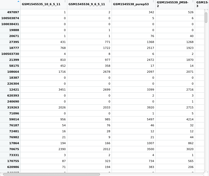
Figure 3.4: View of the count matrix from the DGEList object we created and called x.
Notice that you can use the vertical and horizontal scroll bars to view all of the data. Each row is a gene, denoted by it’s EntrezID and each column is a sample. Each value in this matrix gives the count value for one gene and one sample. Recall also that DGEList specifies that the counts element of the list must be a numeric matrix.
Notice also, that the column names are the file names. The DGEList object was created using the information in the “.txt” files. The function readDGE() has used the file name as the name of each sample because we have not told readDGE() what the sample names are. It has therefore simply used the filenames. This makes logical sense as each file contained the count data for one sample.
The samples dataframe can also be viewed:
View(x$samples)The output should look something like this:
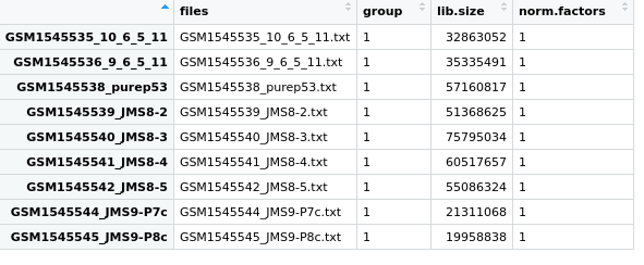
Figure 3.5: View of the samples dataframe from the DGEList object we created and called x.
This is a dataframe where each row is 1 sample, and details of each sample is given in the 4 columns.
filesgives the file names.groupdetails the phenotype group the sample belongs to. As we have not specified this yet, the default1is given for each sample.lib.sizegives the library size. This is the total sum of all counts for that sample.norm.factorsthis gives the normalisation factor for each sample. As we have not calculated any normalisation factors, this is 1 for each sample.
This dataframe also has row names, which are currently the file names of each sample. Again, because we have not told readDGE() what the sample names are, it has used the file names.
Let’s change the row names to be the sample names, instead of the full file name (see Table 3.1).
We can do this by first creating a vector of sample names. You can simply copy and paste the code below into your R script.
samplenames <- c("10_6_5_11", "9_6_5_11", "purep53", "JMS8-2", "JMS8-3",
                 "JMS8-4", "JMS8-5", "JMS9-P7c", "JMS9-P8c")
We can change the row names in the samples dataframe using the rownames() function. This function will give you the row names of a data structure (a dataframe in this instance):
rownames(x$samples) ## [1] "GSM1545535_10_6_5_11" "GSM1545536_9_6_5_11" "GSM1545538_purep53"
## [4] "GSM1545539_JMS8-2" "GSM1545540_JMS8-3" "GSM1545541_JMS8-4"
## [7] "GSM1545542_JMS8-5" "GSM1545544_JMS9-P7c" "GSM1545545_JMS9-P8c"We can see that the row names are the file names as we saw above. To replace these file names with the sample names we can run:
rownames(x$samples) <- samplenamesWe have seen this type of notation before in session 1 (section 1.11). This code assigns the samplenames vector as the row names of the samples dataframe.
Challenge 3.4
- Use the
colnames()function to replace the column names of the count matrix from being file names to sample names. We need to do this because the sample names in thecountsmatrix and thesamplesdataframe should be the same. - The code below creates a factor vector (called
group) that specifies the phenotype group each sample belongs to. It is ordered such that the first element in the vector corresponds to the first row of thesamplesdataframe.
group <- as.factor(c("LP", "ML", "Basal", "Basal", "ML", "LP", "Basal", "ML", "LP")) Replace the group column of the samples dataframe with the group factor vector.
Hint: you will need to use the list subsetting notation we learnt at the start of this session.
- Additional gene annotation information about the genes from our RNA-seq data can be found in the file “Ses3_geneAnnot.tsv”. Read this file in (specifying
stringsAsFactors = FALSE) and add it as another element namedgenesinx(ourDGEListobject).
Hint: the command for adding an element to a list is similar to the command for adding a column to a dataframe. Take a look at Section 1.11 to review how to do the latter.
3.5 Homework
- Subset the first column of the
countmatrix fromx(ourDGEListobject) and ‘save’ (assign) it to a variable calledsample1.
- Find out how many genes had a count of ‘0’.
- Find the total sum of all counts for that sample. Compare this number with the corresponding (first) number in the
lib.sizecolumn from thesamplesdataframe. Is it the same?
Calculate the total sum of the library sizes, using the
lib.sizecolumn from thesamplesdataframe fromx(ourDGEListobject).Using the
genesdataframe fromx(ourDGEListobject), find out how many genes are from chromosome 5.
Hint: you will need to remove rows where the TXCHROM column is NA. Revisit section 2.2 to review missing values.
3.6 Answers
Challenge 3.1
- There are 4 elements of this list.
- For each element -
- Within the first element, there are 2 elements. The first is a vector containing 2 numbers and the second is a vector containing one character type (note there are no ‘scalars’ in R, thus
"a"is a vector with 1 element). - The second element contains 1 element. It is a vector containing two character types.
- The third element contains 2 elements. Within the first element is another list. Within this list there are 2 elements, both being character types. The second element of this nested list is a vector containing one character type.
- The fourth element is a vector containing one character type.
Challenge 3.2
my_list2[[1]]## [1] "a" "b"my_list2[[1]][2]## [1] "b"my_list2[2]## [[1]]
## [1] 1 2 3my_list2[[3]][1,2]## [1] 40my_list2[[3]][1,]## Name Age
## 1 Sally 40my_list2[3]## [[1]]
##    Name Age
## 1 Sally  40
## 2 Andy 32Challenge 3.3
# 1. the vector of cat names
named_list3$cats$name
## [1] "Garfield" "Hello Kitty"# 2. the dog dataframe
named_list3$dogs## name age
## 1 Spot 5
## 2 Snoopy 14# 3. the vector of dog ages
named_list3$dogs$age## [1] 5 14Challenge 3.4
# 1
colnames(x$counts) <- samplenames
# 2
x$samples$group <- group
# 3
geneAnnot <- read.delim("data/Ses3_geneAnnot.tsv", stringsAsFactors = FALSE)
x$genes <- geneAnnot
References
Law, Charity W, Monther Alhamdoosh, Shian Su, Gordon K Smyth, and Matthew E Ritchie. 2016. “RNA-Seq Analysis Is Easy as 1-2-3 with Limma, Glimma and edgeR.” F1000Research 5. Faculty of 1000 Ltd.
Sheridan, Julie M, Matthew E Ritchie, Sarah A Best, Kun Jiang, Tamara J Beck, François Vaillant, Kevin Liu, et al. 2015. “A Pooled shRNA Screen for Regulators of Primary Mammary Stem and Progenitor Cells Identifies Roles for Asap1 and Prox1.” BMC Cancer 15 (1). BioMed Central: 221.