Chapter 2 Session 2
In this session we will learn about:
- how functions work
- missing values
- subsetting data structures
- how to merge two dataframes
2.1 Functions
A function, as the name suggests performs a function. We have already used many functions. For example, the read.delim() function reads in data, the sum() function adds numbers up and the merge() function above merges two dataframes. In this section we will look at functions more formally.
When using a function, brackets (( )) always need to be included after the name of the function. Inputs (technically ‘arguments’) to the function are give within the brackets. You can find out what inputs an argument takes by looking at the help file.
For example, let’s take a look at the rnorm() function help file. This function generates a random number from a normal distribution.
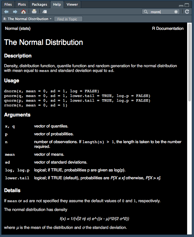
Figure 2.1: rnorm help file.
We can see from the help file that rnorm() takes in 3 arguments:
rnorm(n, mean = 0, sd = 1)The help file also tells us what each of these arguments does:
n   - number of observations. If length(n) > 1, the length is taken to be the number required.
mean - vector of means.
sd - vector of standard deviations.
Challenge 2.1
- Take a look at what the
rnorm()function outputs in the code below. Try using various different inputs to the function then, try to answer the following questions:
- What does
rnorm()do when you only give it one number to themeanandsdarguments? - What happens when you give either argument a vector of numbers?
rnorm(4, mean = 10, sd = 1)## [1] 10.630061 11.198764 9.521584 8.768833rnorm(3, mean = c(100,0), sd = 1)## [1] 99.7151687 -0.9332818 100.4449787- Take a look at the following code:
rnorm(3,1,10)## [1] 9.438640 6.198895 19.857116rnorm(10,1,3)## [1] 5.0067230 3.0310921 -2.1057360 3.6426711 6.1402215 -0.4100198
## [7] -3.0149629 2.6849195 3.8117157 -0.7729955rnorm(3, mean = 10, sd = 0)## [1] 10 10 10rnorm(sd = 10, mean = 0, n = 3)## [1] -2.388429 -3.804495 5.370365How does the order of the arguments you input to the function affect the output? How does the order of the arguments you input affect the output, when you name each argument (along with the input)?
Note: as the function generates a random number, the numbers you will get from running the function will be different to the ones generated above.
2.2 Missing values
Missing values are fairly common in data and in this section, we will look at how to deal with missing values in R. First, let’s read in some data. Recall we use the function read.delim() and tell R not to label words (character type data) as ‘Factors’ using stringsAsFactors = FALSE.
We are using the file “Ses2_genes.tsv” today. This would have been emailed to you before the session. (Alternatively you can download the data from GitHub).
genes <- read.delim("data/Ses2_genes.tsv", stringsAsFactors = FALSE)You can see in the environment tab that this dataframe has 200 rows (observations) and 5 columns (variables). You can also click on the genes entry in the Environment tab (red arrow in Figure 2.2) to display the data in a new window (left):
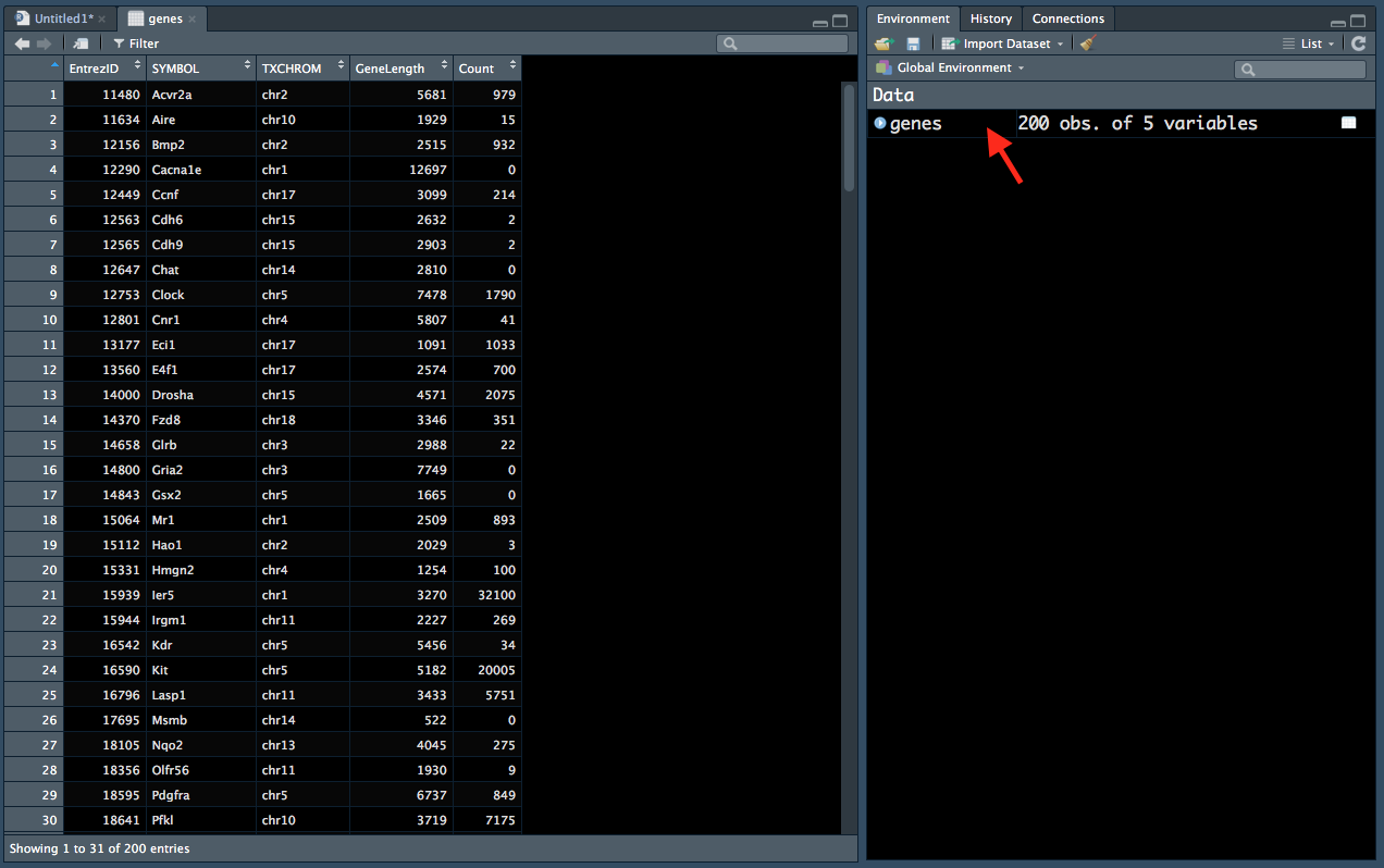
Figure 2.2: Viewing data from the ‘Environment’ tab.
Scrolling down the window, you can see that there are several NA entries. NA denotes a missing value in R.
NA‘s have some interesting behaviour - they are ’contagious’. For example, if we wanted to take the mean of a vector numbers, which includes a NA, the answer is NA. If we think about it, it makes sense that the mean of two numbers and a ‘missing’ number, that could be anything, is NA.
mean(c(2,3,NA))## [1] NALuckily many functions have a na.rm option, where you can tell it to remove NA values:
mean(c(2,3,NA), na.rm = TRUE)## [1] 2.5Later, we will learn how to remove the NA values from our dataframe.
2.2.1 Missing codes
You may have also noticed that in the SYMBOL column, there is a value “missing” on row 3 and a value “Missing” on row 25. These have been used to denote missing values.
It is not uncommon for some people to denote missing values with some character (e.g. “x” or “none” or 999) when performing data entry. It is thus a good idea for us to learn how to deal with this.
We will learn how to do this in the next challenge. This challenge is designed for you to practice how to read help files and gain an understanding of an important computing concept.
Challenge 2.2
- Using the “help” tab in RStudio, find the help file for the function
read.delim(). You will notice that this help file describes several functions but all perform the function of reading data into R. It is not uncommon for functions that perform similar tasks to be grouped together in one help file.
Read the “Arguments” section of the help file and find which argument could be used to tell R that “missing” and “Missing” should be interpreted as a missing value (i.e. a NA).
Read in the file “Ses2_genes.tsv” again but use the argument identified above to tell R that “missing” should be a
NA.Amend your command above so that both “missing” and “Missing” are both interpreted as
NAs.
2.3 Subsetting
Subsetting involves selecting a portion of a data structure and uses square brackets [ ]. There are two main ways to subset a data structure:
- Use indices - data structures are all ordered and ‘numbered’ in R. This means that you can refer to the 4th element in a vector or the element in the 1st row and 3rd column of a dataframe.
- Use logicals - recall that a logical is
TRUEorFALSE. You can use comparisons (e.g. equal to==, greater than>) to determine if each element in your data structure meet your requirements and use this to subset your data.
2.3.1 Subsetting with indicies
Let’s take a look at subsetting vectors first. We can use $ to obtain just one column from the genes dataframe. The output will be a vector.
genes$Count## [1] 979 15 932 0 214 2 2 0 1790 41 1033
## [12] 700 2075 351 22 0 0 893 3 100 32100 269
## [23] 34 20005 5751 0 275 9 849 7175 768 358 234
## [34] 5065 2096 1994 757 0 2310 0 1 0 3091 810
## [45] 30 816 817 1 580 33 0 941 1445 522 2
## [56] 2346 572 431 5797 2 70 1236 966 235 2 3009
## [67] 431 452 2602 3481 99 11857 35 1952 0 706 1317
## [78] 1130 92 0 871 730 3892 3772 20 7 0 756
## [89] 1 210 101 17 21 537 1240 930 1 1 0
## [100] 221 1599 0 67 1 0 315 0 0 739 0
## [111] 0 976 1 715 18636 289 1396 0 101 285 1665
## [122] 47 2 4483 2 363 169 135 0 2 0 11
## [133] 4088 1082 92 0 3888 17 0 0 0 0 0
## [144] 0 0 0 0 0 2442 30 1610 0 0 0
## [155] 16 1 2 0 47 0 1118 0 1 0 2
## [166] 3 22 0 0 0 0 0 0 0 431 0
## [177] 0 16 0 1 0 4 0 0 1 0 0
## [188] 0 0 301 0 0 0 0 0 0 0 0
## [199] 0 59We will assign this to a variable called Counts. Counts is now a variable that refers to a vector containing 200 integers.
Counts <- genes$CountThis will give you the 3rd element of the vector Counts:
Counts[3]## [1] 932This will give you all the elements from the 3rd to the 10th:
Counts[3:10]## [1] 932 0 214 2 2 0 1790 41This will give you the 3rd, 5th and 10th elements:
Counts[c(3,5,100)]## [1] 932 214 221Note that we have used c() within the square brackets. This is because R expects ONE ‘object’ within the square brackets. Thus, if you want to extract several indices, you must give it ONE vector containing the indices of the elements. A vector (e.g. c(3,5,10)) is considered one ‘object’ but the numbers 3,5,10 are considered three different ‘objects’.
Indeed, 3:10, which we used earlier, is actually a vector of the numbers 3 to 10:
3:10## [1] 3 4 5 6 7 8 9 10Lastly, this gives you all the elements EXCEPT the elements 10 through to 200:
Counts[-(10:200)]## [1] 979 15 932 0 214 2 2 0 1790Subsetting a 2 dimensional data structure (e.g. a dataframe or matrix) is similar to subsetting a vector, except you now must specify which rows AND which columns you want. The syntax for the genes dataframe looks like this:
genes[ (which rows you want) , (which columns you want) ]Within the square brackets, you must first tell R which rows you want LEFT of the comma, then which columns you want RIGHT of the comma.
The code below will give you the 3rd to 5th rows of the 2nd and 4th columns. Note that the output is a dataframe.
genes[3:5,c(2,4)]## SYMBOL GeneLength
## 3 missing 2515
## 4 Cacna1e 12697
## 5 Ccnf 3099We could have also done this using the names of the columns. Note that column names are enclosed in quotes signifying that they are of the ‘character’ data type.
genes[3:5,c("SYMBOL","GeneLength")]## SYMBOL GeneLength
## 3 missing 2515
## 4 Cacna1e 12697
## 5 Ccnf 3099If you leave the left side of comma empty, R will give you ALL the rows. If you leave the right side of the comma empty, R will give you ALL the columns.
This will give you the 2nd row and all the columns.
genes[2,]## EntrezID SYMBOL TXCHROM GeneLength Count
## 2 11634 Aire chr10 1929 152.3.2 Subsetting with logicals
If you recall from section 1.6, you can make comparisons in R. The result of a comparison is either TRUE or FALSE:
1 < 2## [1] TRUEComparisons are also vectorised:
genes$Count < 100## [1] FALSE TRUE FALSE TRUE FALSE TRUE TRUE TRUE FALSE TRUE FALSE
## [12] FALSE FALSE FALSE TRUE TRUE TRUE FALSE TRUE FALSE FALSE FALSE
## [23] TRUE FALSE FALSE TRUE FALSE TRUE FALSE FALSE FALSE FALSE FALSE
## [34] FALSE FALSE FALSE FALSE TRUE FALSE TRUE TRUE TRUE FALSE FALSE
## [45] TRUE FALSE FALSE TRUE FALSE TRUE TRUE FALSE FALSE FALSE TRUE
## [56] FALSE FALSE FALSE FALSE TRUE TRUE FALSE FALSE FALSE TRUE FALSE
## [67] FALSE FALSE FALSE FALSE TRUE FALSE TRUE FALSE TRUE FALSE FALSE
## [78] FALSE TRUE TRUE FALSE FALSE FALSE FALSE TRUE TRUE TRUE FALSE
## [89] TRUE FALSE FALSE TRUE TRUE FALSE FALSE FALSE TRUE TRUE TRUE
## [100] FALSE FALSE TRUE TRUE TRUE TRUE FALSE TRUE TRUE FALSE TRUE
## [111] TRUE FALSE TRUE FALSE FALSE FALSE FALSE TRUE FALSE FALSE FALSE
## [122] TRUE TRUE FALSE TRUE FALSE FALSE FALSE TRUE TRUE TRUE TRUE
## [133] FALSE FALSE TRUE TRUE FALSE TRUE TRUE TRUE TRUE TRUE TRUE
## [144] TRUE TRUE TRUE TRUE TRUE FALSE TRUE FALSE TRUE TRUE TRUE
## [155] TRUE TRUE TRUE TRUE TRUE TRUE FALSE TRUE TRUE TRUE TRUE
## [166] TRUE TRUE TRUE TRUE TRUE TRUE TRUE TRUE TRUE FALSE TRUE
## [177] TRUE TRUE TRUE TRUE TRUE TRUE TRUE TRUE TRUE TRUE TRUE
## [188] TRUE TRUE FALSE TRUE TRUE TRUE TRUE TRUE TRUE TRUE TRUE
## [199] TRUE TRUEFor each element in the vector genes$Count, R checks if it is less than 100, then returns either TRUE or FALSE. The output is a vector of logicals.
This can be used to subset in R. We will start with our Counts vector:
Counts[Counts < 100]## [1] 15 0 2 2 0 41 22 0 0 3 34 0 9 0 0 1 0 30 1 33 0 2 2
## [24] 70 2 99 35 0 92 0 20 7 0 1 17 21 1 1 0 0 67 1 0 0 0 0
## [47] 0 1 0 47 2 2 0 2 0 11 92 0 17 0 0 0 0 0 0 0 0 0 0
## [70] 30 0 0 0 16 1 2 0 47 0 0 1 0 2 3 22 0 0 0 0 0 0 0
## [93] 0 0 16 0 1 0 4 0 0 1 0 0 0 0 0 0 0 0 0 0 0 0 0
## [116] 59Counts < 100 will return a vector of 200 logicals, which indicate which elements are less than 100. Putting this inside square brackets will subset Counts such that only the elements that are less than 100 (the TRUE’s) remain.
This is done similarly in 2 dimensional data structures. The command below selects the rows where the genes$Count column equal to 0.
genes[genes$Count == 0,]The code below will output the ROWS where the Count column is equal to 0 and all the COLUMNS (because no input is given after the comma). As there are many rows with a genes$Count of 0, I’ll use the head() function to show just the first 6 rows of the output:
head(genes[genes$Count == 0, ])## EntrezID SYMBOL TXCHROM GeneLength Count
## 4 12290 Cacna1e chr1 12697 0
## 8 12647 Chat chr14 2810 0
## 16 14800 Gria2 chr3 7749 0
## 17 14843 Gsx2 chr5 1665 0
## 26 17695 Msmb chr14 522 0
## 38 19888 Rp1 chr1 9747 0If you add ! to the start of the genes$Count == 0 condition statement, you will get all the rows where genes$Count is NOT equal to 0.
Another way to think about it is that genes$Count == 0 gives you a logical vector of 200 TRUE’s and FALSE’s and ! flips everything such that the TRUE’s become FALSE’s and vice versa.
We do this here and print the first 6 rows of the output:
head(genes[! genes$Count == 0,])## EntrezID SYMBOL TXCHROM GeneLength Count
## 1 11480 Acvr2a chr2 5681 979
## 2 11634 Aire chr10 1929 15
## 3 12156 missing chr2 2515 932
## 5 12449 Ccnf chr17 3099 214
## 6 12563 Cdh6 chr15 2632 2
## 7 12565 Cdh9 chr15 2903 2We can use the $ shortcut to obtain just one column in a dataframe. We can’t do this with matrices - we have to use the [ ] notation instead.
For example, we can create a matrix from our genes dataframe. Recall that a matrix can only hold data of ONE data type - thus we will create a dataframe using just the GeneLength and Count columns of the genes dataframe. The first 6 rows are printed out:
gene_matrix <- as.matrix(genes[,c(4,5)])
head(gene_matrix)
## GeneLength Count
## [1,] 5681 979
## [2,] 1929 15
## [3,] 2515 932
## [4,] 12697 0
## [5,] 3099 214
## [6,] 2632 2If we wanted just the rows where Count was equal to 0, this is the notation we could use:
head(
  gene_matrix[gene_matrix[,2] == 0, ]
)
## GeneLength Count
## [1,] 12697 0
## [2,] 2810 0
## [3,] 7749 0
## [4,] 1665 0
## [5,] 522 0
## [6,] 9747 0We used the [ ] to specify that we want to use the 2nd column of the matrix, which is the Count column. Like above, the == checks if each element in the Count column is 0. There is nothing entered to the right of the comma, indicating that we want all the columns.
Challenge 2.3
- Subset the
genesdataframe to obtain the rows where theCountis less than or equal to 10 and the columnsTXCHROMandCount. - The function
is.na()checks if each element in a vector isNA:
is.na(c(2,5, NA))## [1] FALSE FALSE TRUEUse this function to subset the genes dataframe so that all rows where TXCHROM column is NA is removed.
(Note you do not need to use the subsetted dataframe from question 1 for this question.)
- Using the dataframe from above subset to get only the rows where the
TXCHROMis ‘chr1’ and all columns.
Hint: you can refer to section 1.6 to check how to perform different types of comparisons in R.
2.3.3 %in%
In the last challenge, we used == to obtain the rows where TXCHROM is ‘chr1’. Another way to perform ‘matching’ tasks is with the %in% function.
The following command subsets the rows where TXCHROM is “chr1” or “chr2” and prints out the first 6 rows.
head(
  genes[genes$TXCHROM %in% c("chr1", "chr2"),]
  )
## EntrezID SYMBOL TXCHROM GeneLength Count
## 1 11480 Acvr2a chr2 5681 979
## 3 12156 missing chr2 2515 932
## 4 12290 Cacna1e chr1 12697 0
## 18 15064 Mr1 chr1 2509 893
## 19 15112 Hao1 chr2 2029 3
## 21 15939 Ier5 chr1 3270 32100Challenge 2.4
There is an important difference between == and %in%.
Let’s start by creating a vector of numbers:
vect1 <- c(10,10,5,5,8,8)We check which elements in our vector is equal to 5.
vect1 == 5## [1] FALSE FALSE TRUE TRUE FALSE FALSEThe output is what we would expect.
What if we wanted check which elements are equal to 5 OR 10? We might try something like this, where put the numbers we are checking for in a vector:
vect1## [1] 10 10 5 5 8 8vect1 == c(5,10)## [1] FALSE TRUE TRUE FALSE FALSE FALSEThis isn’t the output we expected.
Let’s try the same task with %in%:
vect1 %in% c(5,10)## [1] TRUE TRUE TRUE TRUE FALSE FALSEThis output IS what we want.
Take a look at the code above and see if you can understand what == does and what %in% does. This challenge is designed to make you think and be difficult.
Hint: The story gets even more interesting if we try to use == to look for four numbers:
vect1 == c(5,10,1,3)## Warning in vect1 == c(5, 10, 1, 3): longer object length is not a multiple
## of shorter object length## [1] FALSE TRUE FALSE FALSE FALSE FALSEThis warning message may seem a bit cryptic. The ‘longer’ object it is referring to is vect1 which has 6 elements. The shorter object it is referring to is c(5,10,1,3), which has 4 elements. Thus, it is saying that 6 is not a multiple of 4. The reason R wants the longer object to be a multiple of the shorter one, is key to understanding what is happening when we use ==.
2.4 Merge
Two dataframes can be combined with the merge() function.
For example, let’s say we have two dataframes (dataframe1 and dataframe2), each containing different information about 3 genes:
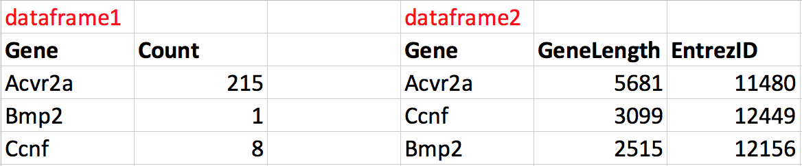
Figure 2.3: The two dataframes to merge.
We can merge these dataframes together into one dataframe that contains all the information about genes. Notice that the order of the genes is not the same in the two dataframes. During the merge we want R to match each row according to the Gene column in each dataframe such that the correct information is added to the correct row. The result would have 4 columns, 3 rows and the correct information along each row.
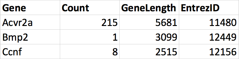
Figure 2.4: The two dataframes merged.
Let’s practice merging on the files “Ses2_genes.tsv” and “Ses2_geneNames.tsv”. “Ses2_genes.tsv” contains gene EntrezIDs, gene symbol, gene chromosome, gene length and their count value. “Ses2_geneNames.tsv” contains gene names and their corresponding EntrezIDs.
First we will read in both files:
genes <- read.delim("data/Ses2_genes.tsv", stringsAsFactors = FALSE)
gene_names <- read.delim("data/Ses2_geneNames.tsv",
                         stringsAsFactors = FALSE)
What we want to do now, is to merge the two dataframes into one dataframe with 6 columns, containing the information from both dataframes. We also want to make sure that when R merges the dataframes, the correct information is added to the correct row. You will notice that both the genes and gene_names dataframes have a column giving the EntrezIDs. This column can be used as the “index” or “ID” column to make sure the correct information is added to each row. We can do this by telling merge() to match rows in the two dataframes using EntrezIDs during the merge.
merge() has the following syntax:
merge(
  x =    # name of the first dataframe to merge
  y =    # name of the second dataframe to merge
  by.x = # name of the column to match, in the first dataframe
  by.y = # name of the column to match in the second dataframe
)
Thus, to merge our two dataframes, using the EntrezID column of each dataframe to match rows, we can use:
genes2 <- merge(x = genes, y = gene_names,
                by.x = "EntrezID", by.y = "ENTREZID")

head(genes2)
## EntrezID SYMBOL TXCHROM GeneLength Count
## 1 11480 Acvr2a chr2 5681 979
## 2 11634 Aire chr10 1929 15
## 3 12156 missing chr2 2515 932
## 4 12290 Cacna1e chr1 12697 0
## 5 12449 Ccnf chr17 3099 214
## 6 12563 Cdh6 chr15 2632 2
## GENENAME
## 1 activin receptor IIA
## 2 autoimmune regulator (autoimmune polyendocrinopathy candidiasis ectodermal dystrophy)
## 3 bone morphogenetic protein 2
## 4 calcium channel, voltage-dependent, R type, alpha 1E subunit
## 5 cyclin F
## 6 cadherin 6You may have noticed that there are 200 rows in the genes dataframe but 290 rows in the gene_names dataframe. This means that there are more genes in the gene_names dataframe than there are in the genes dataframe. This means that there are a few ways to merge the two dataframes. We can either keep all rows from both dataframes, keep only rows where there is a corresponding “index” value in both dataframes or keep only rows from one of the two dataframes.
We can specify which rows to keep using the following additional arguments in merge():
merge(
  x =     # name of the first dataframe to merge
  y =     # name of the second dataframe to merge
  by.x =  # name of the column to match, in the first dataframe
  by.y =  # name of the column to match in the second dataframe
  all.x = # logical. If TRUE, keep all rows from the first dataframe,
          # even if does not have a matching row in the second dataframe
  all.y = # logical. If TRUE, keep all rows from the second dataframe,
          # even if does not have a matching row in the second dataframe
)
By default, merge() will only keep rows that have corresponding “index” values in both dataframes.
Challenge 2.5
Merge the two dataframes again, but this time keep all rows from both dataframes.
2.5 Homework
- Subset your
genesdataframe to obtain the rows 5 to 10, 45 and 72 and all the columns EXCEPT column 4. - Subset your
genesdataframe to obtain only rows where genes with the symbol is “Rab18”, “Ripk1” or “Xpr1” and all the columns. - Read in the tsv file “Ses2_PFAM.tsv” (remember to include
stringsAsFactors = FALSE). This file gives the EntrezID next to the Pfam code for all our genes.- Remove all rows where the Pfam code is
NA - Merge this dataframe to
genes, keeping all rows from both dataframes
- Remove all rows where the Pfam code is
2.6 Answers
Challenge 2.1
- If you provide
rnorm()with a vector of inputs to either themeanorsdargument, it will use each element in that vector for successive random numbers generated and recycle the vector if it is shorter than the number of random numbers required.
Thus, the following code:
rnorm(3, mean = c(100,0), sd = 1)will generate 3 random numbers from the following normal distributions, in order:
1. mean of 100 and sd of 1
2. mean of 0 and sd of 1
3. mean of 100 and sd of 1- If you do not provide the name of the argument,
rnorm()will use the first number provided as the argument ton, the second number provided as the input tomeanand the third number provided as the input tosd.
Thus, rnorm(3,1,10) generates 3 random numbers from a normal distribution with a mean of 1 and a standard deviation of 10 and rnorm(3,10,1) will generate 3 random numbers from a normal distribution with a mean of 10 and a standard deviation of 1.
If you give the argument name with the input, it does not matter what order you provide the inputs.
Challenge 2.2
- The
na.stringsargument.
genes <- read.delim("data/Ses2_genes.tsv", stringsAsFactors = FALSE,
                    na.strings = "missing")
genes <- read.delim("data/Ses2_genes.tsv", stringsAsFactors = FALSE,
na.strings = c("missing", "Missing"))The reason you need to give c("missing", "Missing") to the argument na.strings is quite complex. First, R expects only one “thing” (the technical term is “object” and we will discuss this more indepthly next session) for each argument. Notice that for the other arguments of read.delim(), only one “object” as been given. "missing", "Missing" is interpreted as two “objects” (two character values), whereas c("missing", "Missing") is one “object” (one vector that contains two values).
The other concept to note here is that , has a special meaning in functions. It is used to separate each argument. Thus, the comma in "missing", "Missing" causes R to interpret the "Missing" after the comma to be another argument to read.delim(). However, there is no argument called "Missing" and further, arguments should NEVER have quotes around them. The error you get Error in !header : invalid argument type is essentially saying this - arguments should not be characters.
Challenge 2.3
- This code obtains rows where
Countis less than or equal to 10 and prints the first 6 rows usinghead():
head(genes[genes$Count <= 10,])## EntrezID SYMBOL TXCHROM GeneLength Count
## 4 12290 Cacna1e chr1 12697 0
## 6 12563 Cdh6 chr15 2632 2
## 7 12565 Cdh9 chr15 2903 2
## 8 12647 Chat chr14 2810 0
## 16 14800 Gria2 chr3 7749 0
## 17 14843 Gsx2 chr5 1665 0- This code removes all rows where the
TXCHROMcolumn has a NA value (keeping all columns) and prints the first 6 rows:
head(genes[! is.na(genes$TXCHROM),])## EntrezID SYMBOL TXCHROM GeneLength Count
## 1 11480 Acvr2a chr2 5681 979
## 2 11634 Aire chr10 1929 15
## 3 12156 missing chr2 2515 932
## 4 12290 Cacna1e chr1 12697 0
## 5 12449 Ccnf chr17 3099 214
## 6 12563 Cdh6 chr15 2632 2- First we save the dataframe from the above as a variable called
genes_noNA, then we subset to get only the rows whereTXCHROMis ‘chr1’. Again we only print the first 6 rows of this output.
genes_noNA <- genes[! is.na(genes$TXCHROM),]

head(genes_noNA[genes_noNA$TXCHROM == "chr1",])
## EntrezID SYMBOL TXCHROM GeneLength Count
## 4 12290 Cacna1e chr1 12697 0
## 18 15064 Mr1 chr1 2509 893
## 21 15939 Ier5 chr1 3270 32100
## 31 18777 Lypla1 chr1 2433 768
## 36 19775 Xpr1 chr1 7651 1994
## 38 19888 Rp1 chr1 9747 0Challenge 2.4
What == does is compare vect1 with c(5,10) one by one. Since c(5,10) only has two elements, R repeats this shorter vector until it is the same length as the longer vector. This is called ‘recycling’.
Thus, the comparisons being made is the top row with each corresponding value in the bottom row, with the result being shown in the third row:
10     10    5    5     8     8

5      10    5    10    5    10

FALSE TRUE TRUE FALSE FALSE FALSE
R gives you a warning whenever the length of the shorter vector is NOT a multiple of the longer vector.
When there were 4 elements in the shorter vector, it was not repeated a whole number of times - it was repeated 1.5 times. The comparisons being made between vect1 and c(5,10,1,3) are:
10     10    5    5     8     8

5      10    1    3     5    10

FALSE TRUE FALSE FALSE FALSE FALSE
%in% simply performs matching and does not take order of the two vectors into consideration. It checks whether the values in vect1 matches either number in c(5,10). It thus gives us the result we expect.
Challenge 2.5
genes2 <- merge(x = genes, y = gene_names,
                by.x = "EntrezID", by.y = "ENTREZID",
                by.x = TRUE, by.y = TRUE)